The Crank-Nicolson method is a popular finite difference numerical method for solving partial differential equations (PDEs) – which are equations with two or more independent variables. The 1-D heat equation below has two independent variables, the time variable, t, and the spatial dimension, x.

The question becomes, how does the Crank-Nicolson method to solve PDEs compare to included solvers in various programming languages, e.g. MATLAB?
MATLAB contains various solvers for solving ordinary differential equations (equations with only one independent variable), e.g. ‘ode23’ and ‘ode45’; and at least one solver that solves 1-D PDEs (parabolic and elliptic) – the ‘pdepe’ solver. On my quest to see which of the two yielded quicker results – the ‘pdepe’ solver vs Crank-Nicolson finite difference method, below is a brief summary of this evaluation.
Case study: The classic 1-D rod example, where one end is held at a fixed elevated temperature (for this example, I used 100 deg C), and the other end is also held at a fixed temperature, but at a cooler value (say, 50 deg C). The initial condition of the rod, that is the temperature of the internal nodes of the rod are set to 0 deg C at t = 0. At t > 0 the rod is subjected to the temperature extremes on either end. Fourier’s Law of heat conduction goes into full force… errr conduction, and is used to solve the PDE problem.
This write-up is not meant to provide a heavy background on the mathematics, or Fourier’s law of heat conduction, but rather a quick overview of the difference in results from two methods used to analyze the problem. MATLAB code for both methods is provided at the end via GitHub links, which contains mathematical background and derivations.
All solution mesh parameters are equal for both cases.
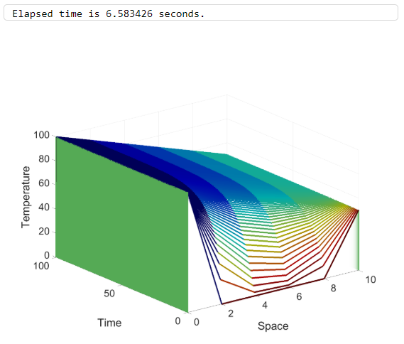
Case one: Solving the 1-D heat equation via the Crank-Nicolson finite-difference numerical method
Discussion of results: Consulting the plot, and focusing on node 2 (element / column 3 in the Temp. solution matrix), x = 4 cm, it is observed that temperature increases at a steady rate, and reaches a steady-state temperature of ~33 deg C at approximately 24 seconds after being subjected to the boundary conditions (T = 100 deg C at the left end of the rod, and T = 50 deg C at the right end of the rod, both ends are fixed for all time). The same conclusion can be drawn for the other nodes in the system, with transient times also being close to equal.
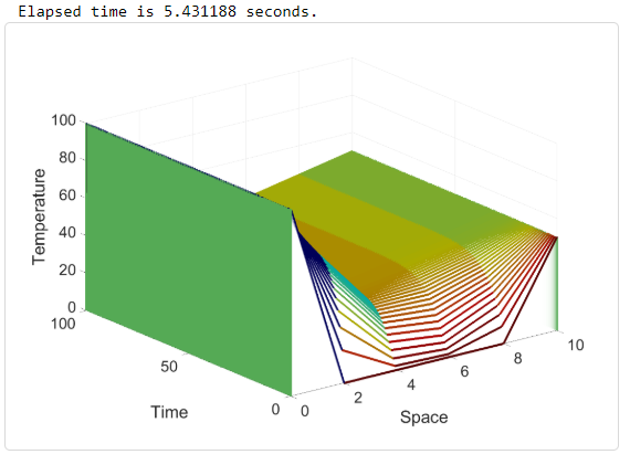
Case two: Solving the 1-D heat equation via the MATLAB pdepe partial differential equation solver

Discussion of results: Consulting the plot, and focusing on node 2 (element / column 3 in the Temp. solution matrix), x = 4 cm, it is observed that temperature increases at a steady rate, and reaches a steady-state temperature of ~79 deg C at approximately 47 seconds after being subjected to the boundary conditions (T = 100 deg C at the left end of the rod, and T = 50 deg C at the right end of the rod, both ends are fixed for all time). The same conclusion can be drawn for the other nodes in the system, with transient times being close to equal for all nodes.
Summary: The computing time to solve is negligible (5.4 sec vs 6.6 sec) for this simple case, but this may grow in proportion to the complexity of the system being analyzed. What’s more important is the solution; notice the ragged solution in case one – this of course can be improved by refining the mesh. Case two also exhibits this ragged behavior, but smooths out much quicker. This lack of mesh refinement caused for a large delta in the transient times (time to reach steady-state), with case one having a transient time of 24 seconds vs case two of 47 seconds.
In any case, it should be noted that the ‘pdepe’ solver does a great job in solving the PDE equation and will suffice in solving a 1-D problem; however, if you are new to solving PDEs numerically, this may seem like you are throwing something into a black box. The Crank-Nicolson method does a great job in demystifying PDEs and breaking down abstract terms into their most simplest elements. It is therefore wise to have an understanding of both methods.
Happy solving!
GitHub link to code used in case one:
GitHub link to code used in case two:
… Coming soon… working through some source control issues… ejr 7/23/21
I must thank you for the efforts youve put in penning this site. I am hoping to check out the same high-grade blog posts by you in the future as well. In fact, your creative writing abilities has motivated me to get my very own blog now 😉