
Solving partial differential equations is hard, luckily we have numerical methods to help us break apart abstract mathematical concepts into the most simplest elements – the Crank-Nicolson method allows for a simple way to solve parabolic PDEs.
Let’s look at the classic example of a one-dimensional rod that is subjected to two opposing temperatures on either end, hot and cold. How do we determine the temperature distribution along the rod as time progresses? In comes, partial differential equations.
We start our journey with the heat-conduction equation:

What is this equation telling us… in English? – The rate at which temperature at a point changes with respect to time, is equal to the rate of the rate of change of that point with respect to space times a constant k, representing the material’s thermal diffusivity.
Remember: Where’s there’s curvature in space, there’s change in time. So, the right-hand side is telling us how the temperature distribution curves as we move across space.
Solving PDEs using analytical methods is hard! Luckily, we have numerical methods. The Crank-Nicolson is one such method, which happens to be second-order accurate in both space and time – which is good. Let’s consider a computational molecule for the Crank-Nicolson method:
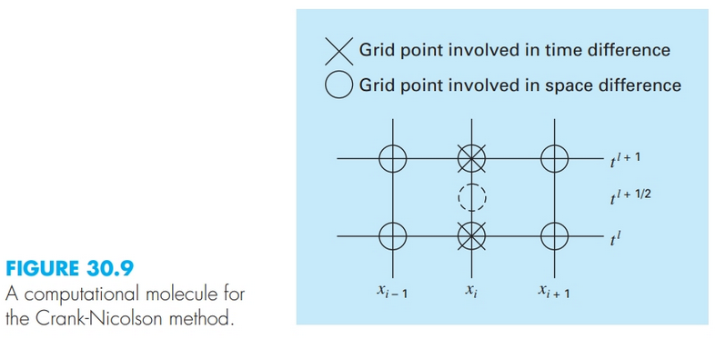
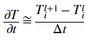
The temporal first derivative is approximated at the center (dashed circle, representing the center node):
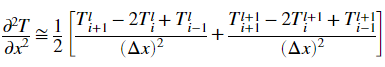
The spatial second derivative is determined at the midpoint by averaging the difference approximations at the beginning and end of the time increment:
We can now use the above approximations of the hairy partial derivative terms to make our life a bit easier!
The rest of the problem involves some algebraic manipulation, applying boundary conditions, and setting our initial conditions and we are on our way to solving the heat equation. Which brings me to my next point. What does it mean to SOLVE an equation made up of partial derivatives? Well, simply, it’s a series of spatial distributions corresponding to the state (temperature) of the node at each time.
You can find a flowchart outlining how to go about how to create a computer program to solve this PDE, pseudocode, and MATLAB program code solving the problem here: https://github.com/mannyjrod/Solving_Parabolic_PDEs
Finally, remember that our entire world can be modeled using mathematics — this is the beauty of it all!